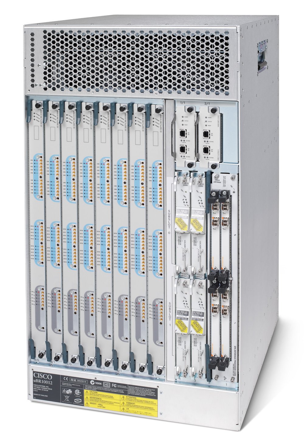
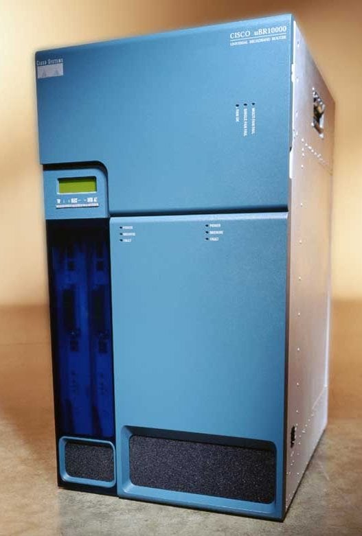
Cable modem termination systems (CMTSs) can report a variety of operating parameters to the end user. For example, CMTSs that use Broadcom BCM3137, BCM3138, or BCM3140 or Texas Instruments TNETC4522 series upstream burst receivers can provide an "upstream SNR" estimate. This function is a very useful tool, but it has resulted in much confusion. It is not unusual for a cable company's network operations center (NOC) staff to report an alarm condition when the reported upstream signal-to-noise ratio (SNR) of the CMTS drops below a defined threshold. A headend technician follows up by checking the upstream RF performance with a spectrum analyzer or similar test equipment, only to find that everything appears normal.
Data personnel in the NOC insist there must be a problem, while outside plant technicians see nothing amiss on their test equipment. What is going on here?
The discrepancy occurs from a lack of understanding about just what the CMTS upstream SNR estimate is - and what it is not.
Further confusion comes from the fact that cable modems and digital set-top boxes (STBs) can provide digitally modulated signal operating parameters such as RF signal level and SNR. These are downstream parameters at the customer premises, not upstream parameters as is sometimes incorrectly assumed. In addition, test equipment used by cable operators to characterize digitally modulated signals can measure downstream - and in some cases upstream - modulation error ratio (MER). Some of these instruments call this parameter SNR.
Also, because of the time-shared nature of the upstream, most of today's CMTSs can measure parameters on a per-channel basis or a per-cable-modem basis. Per-channel measurements provide an average of all cable modems or simply a snapshot of the most recently active cable modem(s). It is important to distinguish which type of measurement is presented.
This paper provides a background on several signal quality metrics applicable to CMTS and cable network operation and how they relate to overall performance. The CMTS upstream SNR and cable modem or STB downstream SNR estimates are explained. Noise, as discussed in this paper and unless defined otherwise, refers to additive white Gaussian noise (AWGN), or simply white noise, also known as thermal noise. Interference such as narrowband ingress and burst or impulse noise is usually treated separately.
First, what the CMTS upstream SNR estimate is not: the SNR estimate from a cable modem or CMTS is not the same thing as the carrier-to-noise ratio (CNR) that one measures with a spectrum analyzer.
Here is what the upstream SNR estimate is: an operating parameter provided by the upstream burst receiver used in DOCSIS® CMTSs. Similar information for downstream signals is provided by the quadrature amplitude modulation (QAM) receiver in a cable modem or STB. The SNR estimate, which is derived after the data is demodulated, is more accurately called receive modulation error ratio (RxMER), a term recently defined in the DOCSIS MIB. RxMER includes the effects of the cable network downstream or upstream noise floor, in-channel frequency response (including amplitude tilt and ripple, group delay variation, and micro-reflections), oscillator phase noise, receiver imperfections, and all other impairments that affect the receive symbol constellation. Because it measures the end-to-end performance of the communications link, RxMER is useful for tracking long-term system performance trends.
Interestingly, it is not unusual to have a reported low downstream or upstream RxMER number, yet find the measured CNR and signal levels to be just fine. Why? Because one or more impairments that cannot be seen on a spectrum analyzer - poor in-channel frequency response, including group delay variation and micro-reflections, and even upstream data collisions - may be the cause of the low reported RxMER.
This paper discusses the terms listed in Table 1.
Table 1. Terminology for Various SNR Ratio Concepts
Abbreviation
Term
Definition
Units
CNR (or C/N)
Carrier-to-noise ratio
The ratio of carrier or signal power to the white-noise power in a specified bandwidth, as measured on an RF spectrum analyzer or similar equipment.
dB
C/N0
Carrier-to-noise -density ratio
The ratio of carrier or signal power to white-noise spectral density.
dB-Hz
CNIR
(or C/(N+I))
Carrier-to-noise-plus-interference ratio
The ratio of carrier or signal power to the total noise power (including white noise and interference) in a specified bandwidth, as measured on an RF spectrum analyzer or similar equipment.
dB
ES/N0
Energy-per-symbol to noise-density ratio
In digital modulation, the ratio of the average energy of a QAM symbol to the white-noise spectral density.
dB
EVM
Error vector magnitude
The ratio of RMS constellation error magnitude to peak constellation symbol magnitude.
Percent
MER
Modulation error ratio
The ratio of average signal constellation power to average constellation error power.
dB
RxMER
Receive modulation error ratio
The MER as measured in a digital receiver after demodulation, with or without adaptive equalization.
dB
SNR
(or S/N)
Signal-to-noise ratio
(a) A general measurement of the ratio of signal power to noise power.
(b) In a specific context, a measurement of the ratio of signal power to noise power made at baseband before modulation or after detection or demodulation.
dB
TxMER
Transmit modulation error ratio
The MER produced by a transmitter under test, as measured by an ideal test receiver.
dB
CNR and SNR from a Telecommunications Industry Perspective
Some of the confusion mentioned in the introduction arises from the fact that in the world of telecommunications outside the cable industry, the terms SNR and CNR are often used interchangeably. According to Roger L. Freeman's Telecommunications Transmission Handbook, "The signal-to-noise ratio expresses in decibels the amount by which a signal level exceeds its corresponding noise." Another reference, Tektronix's Measuring Noise in Video Systems, says "In the most general case, SNR is expressed as the ratio of RMS (root mean square) signal level, SRMS, to the RMS noise, NRMS, (SNR = SRMS/NRMS)." [Eq. 1]
Both of the previous SNR definitions can easily be applied to RF CNR measurements (after all, a carrier is a "signal") as well as baseband SNR measurements (baseband video and audio are "signals," too). If the specific measurement is not clearly defined, it is difficult to know whether SNR refers to a baseband or RF parameter. This paper distinguishes between SNR and CNR. In the subsequent sections each term is defined and explained, and the distinction is illustrated following usage in the cable industry.
CNR and SNR from a Cable Industry Perspective
Modern Cable Television Technology, 2nd Ed., states, "Carrier-to-noise ratio (C/N) is defined as follows:
[Eq. 2]
where c and n are the scalar power levels of the carrier and noise, respectively."1
When measuring CNR on a spectrum analyzer with thermal noise underlying the carrier, one actually is measuring not C/N but, more precisely, (C+N)/N = 1 + C/N. This distinction is not normally a concern unless the CNR is very low - say, single-digit decibel (dB) values, as we will see later.2
The cable industry has long used CNR and SNR to represent quite different measurement parameters, one in the RF domain (Figure 1) and the other in the baseband domain (Figure 2). CNR is applied to the transmitted over-the-cable RF waveform, whereas SNR refers to the video and audio signal prior to modulation for broadcast, or after demodulation of the RF waveform at the receiver.
Figure 1. RF CNR Measurement (as detected in the test equipment resolution bandwidth)
Figure 2. Baseband SNR Measurement
Analog Video CNR in Cable Networks
Consider CNR, which is generally accepted to be a predetection measurement - that is, one made at RF. When only analog TV channels were carried on cable networks, CNR was understood to be the difference, in decibels, between the amplitude of a TV channel visual carrier3 and the root mean square (RMS) amplitude of system noise in a specified noise power bandwidth. In this application, noise power bandwidth is normally specified as the modulation bandwidth, which is approximately equal to the bandwidth of the baseband modulating signal. It is common practice to express power in terms of RMS voltage across a nominal resistance. For example, NCTA Recommended Practices for Measurements on Cable Television Systems defines 0 dBmV (decibels referenced to one millivolt) as the power of a signal of 1 millivolt RMS in 75 ohms, or 13.33 nanowatts = -48.75 dBm.
According to the Federal Communications Commission's (FCC's) cable regulations in §76.609 (e), system noise is the "total noise power present over a 4-MHz band centered within the cable television channel." This latter definition is applicable only to analog National Television System Committee (NTSC) TV channel CNR measurements, and defines the approximate bandwidth of the baseband video that modulates the channel visual carrier.
The FCC does not actually use the term CNR in the rules. §76.605 (a)(7) states "The ratio of RF visual signal level to system noise shall...not be less than 43 decibels." That definition is more or less in line with the general definition of SNR, although it is understood in this specific instance to mean CNR. Even though the FCC's cable rules mandate a minimum CNR of 43 dB, good engineering practice targets end-of-line analog TV channel CNR in the 46 to 49 dB range. More on this topic appears later in this paper.
Analog Video SNR in Cable Networks
What about SNR? SNR is, in cable industry vernacular, a premodulation (at the transmitter or modulator) or postdetection (at the receiver) measurement - one made on a baseband signal such as video or audio. The previously mentioned Tektronix application note says: "In video applications, however, it is the effective power of the noise relative to the nominal luminance level that is the greater concern." It goes on to define video SNR in decibels as:
SNR = 20log(LNOMINAL/NRMS) [Eq. 3]
where LNOMINAL has a value of 714 millivolts peak to peak (100 IRE units) for NTSC or 700 mV peak to peak for PAL. These luminance values do not include sync.
Equation 3 simply states that baseband video SNR is the ratio of the peak-to-peak video signal, excluding sync, to the noise within that video signal. The noise is measured in a bandwidth defined by a combination of low-pass, high-pass, and weighting filters. These filters limit the measured noise to a bandwidth that is roughly the same as the video signal and may be used to remove certain low-frequency noise from the measurement. Weighting filters are used to simulate the eye's response to noise in the TV picture. Various standards such as RS-170A, RS-250B, and NTC-7 specify the characteristics of filters that are used in baseband video SNR measurements.
To recap: CNR is a predetection measurement performed on RF signals. It is the difference, in decibels, between carrier power and noise power in the RF transport path only - for instance, a coaxial cable distribution network or a standalone device such as an upconverter or headend signal processor. As such, CNR is ideal for characterizing network or individual device impairments. SNR, when applied to analog video or audio signals, is a premodulation or postdetection measurement performed at baseband. It is equal to the ratio of the peak-to-peak baseband signal to the noise within that signal (refer to Figure 1). SNR includes noise in the original signal - say, noise in the video from a TV studio camera - as well as noise contributions from the transmitter or modulator, transport path, receiver, and demodulator. It is ideal for characterizing end-to-end performance - the overall picture quality seen by the end user, in the case of baseband video SNR.
Discrete Versus Modulated Signals and Carrier-to-Noise Density Ratio
A measurement that is closely related to CNR is carrier-to-noise-density ratio (C/N0), defined as the ratio of carrier or signal power (in watts) to the underlying white-noise power spectral density (in watts/Hz). Noise power spectral density N0 is the noise power in a 1 Hz bandwidth - that is, watts per Hz. Because of the impracticality of making a 1 Hz bandwidth noise power measurement, noise power spectral density is usually measured in a larger, more convenient bandwidth - the test equipment resolution bandwidth (RBW) - or, to be more precise, the equivalent noise bandwidth of the RBW filter. The measured value in watts is then divided by the test equipment resolution bandwidth in Hz, which yields the power (in watts) in a 1 Hz bandwidth. If the noise power measurement is in dBmV, subtract 10log(RBW in Hz) from the measured value to get the 1 Hz bandwidth equivalent, also in dBmV.
Taking the ratio of units shows that C/N0 has units of Hz:
[Eq. 4]
In decibels, C/N0 is expressed in dB-Hz, which means "decibels referenced to one Hz." Because C/N0 is not unitless like other SNR and CNR metrics, care must be taken to reference the noise measurement to a 1 Hz noise bandwidth.
C/N0 is especially useful for measuring the CNR of a narrowband signal such as an unmodulated or continuous wave (CW) carrier. Consider a spectrum analyzer capture of a CW signal in a white-noise background, with the analyzer RBW set to 100 kHz. Assume that placing the analyzer marker on the CW signal indicates an amplitude of -10 dBmV, and moving the marker to the displayed noise floor shows -40 dBmV. Be careful - this noise reading is not in dBmV/Hz, but represents the noise power in the analyzer RBW as mentioned previously, giving a spectral density of -40 dBmV/(100 kHz). To convert to a 1-Hz bandwidth, subtract 10log(100,000 Hz) = 50 dB-Hz. So the noise density is actually -40 dBmV - 50 dB-Hz = -90 dBmV/Hz. Some spectrum analyzers have a marker noise function that provides automatic readings in a 1-Hz bandwidth, eliminating the need for this conversion. The true C/N0 is then (using dB quantities):
To convert C/N0 to CNR in a given bandwidth B, we use
CNR = C/N = C/(N0B) [Eq. 6]
So in decibels, to convert C/N0 to CNR, subtract 10log(B). The CW signal in this example would have a CNR in a 6 MHz bandwidth (using decibel quantities) of
This example illustrates an important principle when measuring a mix of discrete signals (CW or any signals that are much narrower than the RBW of the analyzer) and spread signals (such as noise or modulated signals that are much wider than the analyzer RBW). The spectrum analyzer marker simply measures power in the RBW. For a narrowband signal, this measurement equals the carrier power. For noise, it gives the density referenced to the RBW. Scale to a 1-Hz bandwidth to get C/N0, and scale to a desired bandwidth B to get CNR.
Digitally Modulated Signal CNR
What about CNR measurement of digitally modulated signals on a cable plant? The DOCSIS Radio Frequency Interface Specification states an assumed minimum 35-dB CNR for downstream digitally modulated signals. If the network analog TV channel CNR is maintained in the 46-dB or higher range, in most cases, there will be little or no problem complying with the DOCSIS assumed minimum for downstream digitally modulated signals. The DOCSIS assumed minimum upstream CNR for digitally modulated signals is 25 dB. Carrier power - the "C" in CNR - is the average power level of the digitally modulated signal, often called digital channel power. It is measured in the full occupied bandwidth of the signal; for example, 6 MHz for a North American DOCSIS downstream signal.
Is a Digitally Modulated Signal a "Carrier"?
Quadrature amplitude modulation results in a double-sideband, suppressed-carrier RF signal. Before modulation is applied, the unmodulated signal is certainly a carrier - a CW carrier. But when modulation is applied, the carrier is suppressed. From one perspective, it could be correctly argued that the "haystack" of a QAM signal is not a carrier - it is just an RF signal - because the carrier is suppressed. From another perspective, it is legitimate to argue that a QAM signal "carries" information because its modulation was impressed on a carrier frequency. The underlying carrier can be recovered and tracked by a digital receiver. In fact, a QAM signal is cyclostationary - its carrier can be regenerated and observed on a spectrum analyzer by first passing the QAM signal through a nonlinearity such as 4th power. To minimize confusion with baseband signals and to follow common industry parlance, this paper refers to digitally modulated RF signals as "modulated carriers," or simply "carriers."
To measure the white noise - the "N" in CNR - underlying a digitally modulated signal, a noise power bandwidth (also called equivalent noise bandwidth or effective bandwidth) equal to the symbol rate should be used. The noise measurement should be performed when the signal is not present, or in an empty band near the signal. Tables 2 and 3 summarize noise power bandwidth values for DOCSIS downstream and upstream channels.
Table 2. Noise Power Bandwidth for DOCSIS Downstream Channels
Channel RF (Occupied) Bandwidth
Symbol Rate Rs
Noise Power Bandwidth (approximate)
6 MHz
5.056941 Msym/sec
5.06 MHz
6 MHz
5.360537 Msym/sec
5.36 MHz
8 MHz (Euro-DOCSIS)
6.952 Msym/sec
6.95 MHz
Table 3. Noise Power Bandwidth for DOCSIS Upstream Channels
1In the DOCSIS 2.0 Physical Media Dependent Sublayer Specification, the term "modulation rate in kHz" is used instead of symbol rate in kilosymbols per second. This definition encompasses both TDMA and S-CDMA transmission.
Downstream Digitally Modulated Signal CNR - An Example
Assume that a cable network has been designed to provide a downstream end-of-line CNR of 46 dB with +15 dBmV subscriber tap levels for analog TV channels, and a downstream 64-QAM DOCSIS digitally modulated signal is carried at -10 dBc. Thus the digital channel power of the 64-QAM signal at the tap spigot will be +5 dBmV, or 10 dB lower than the +15 dBmV analog TV channel levels. What is the 64-QAM signal CNR? It is not 36 dB as one might first assume.
Because analog TV channel CNR is 46 dB at the tap spigot, the noise-floor amplitude NNTSC for the analog channels is +15 dBmV - 46 dB = -31 dBmV (4-MHz noise power bandwidth for analog NTSC TV channels). To determine the 64-QAM signal CNR, we have to first calculate what the noise-floor amplitude is for that QAM signal, based on a noise power bandwidth equal to its symbol rate. For DOCSIS 64-QAM signals, the symbol rate is 5.056941 Msym/sec, so the noise power bandwidth is 5.06 MHz (refer to Table 2). From this, we can calculate the noise-floor amplitude N64-QAM for the QAM signal with the equation
The 64-QAM signal CNR is +5 dBmV - (-29.98 dBmV) = 34.98 dB.
The CNR of the digitally modulated signal is degraded by more than the 10-dB reduction in signal level because the wider noise bandwidth in the digital signal case allows more AWGN through to the demodulator.
ES/N0 and CNR of a Digitally Modulated Signal
ES/N0 is the most prevalent parameter used in digital communications to represent the SNR of a signal. It is defined as the ratio of the average energy ES per QAM symbol to the noise power spectral density N0 with the noise assumed white. It is a unitless ratio and is normally expressed in dB. Energy per symbol is equal to the average power - that is, the energy in 1 second - of the signal divided by the number of symbols in 1 second.
How can we reconcile ES/N0 with CNR? If we multiply the numerator and denominator by the symbol rate RS, we get:
[Eq. 9]
(assuming no synchronous code-division multiple access [S-CDMA] spreading, which we discuss later). This equation tells us why the measurement of CNR for digitally modulated signals typically uses the noise power bandwidth equal to the symbol rate: It results in CNR being equal to ES/N0.
QAM Spectrum Basics
Consider what a QAM signal spectrum looks like, and how we can read the signal power, noise power, and CNR from the spectrum display.
First, some background on transmit and receive filters. Figure 3 shows a communications system, which represents an upstream or downstream cable data network. Both the transmitter and receiver contain "matched filters." The purpose of the transmit matched filter is to band-limit the transmitted spectrum so that it will not interfere with adjacent channels. The purpose of the receive matched filter is to select the desired channel and to reject noise. The "matched" property of the filters implies that they have identical frequency magnitude response .
A time-invariant system such as a filter can be characterized by its impulse response h(t) or by its frequency response , which comprise a Fourier transform pair. The asterisk on the receive filter in Figure 3 indicates that the receive matched filter exhibits complex conjugation of its frequency response, or equivalently, time-reversal of its impulse response, relative to the transmit filter. However, this property is not of practical importance in cable systems because the filters are time-symmetric.
Matched filtering is known to maximize receive SNR in the presence of white noise. The cascade of the two matched filters gives the "full" magnitude response . A signal having this full magnitude response is seen only at the output of the receive matched filter, inside of the receiver, and is not normally visible to an outside observer. However, the full-filter response is important in that it is designed to have the Nyquist property, described in the next section.
Figure 3. General Digital Communications System Showing Matched Filters in Transmitter and Receiver
The signal marked "Tx Signal" in Figure 3 represents the actual transmitted signal that is observable on the cable plant. (We are neglecting upconversion and downconversion to/from RF and are dealing only with "complex envelopes" in this discussion.) Because the scrambler guarantees that the QAM symbols affecting the transmit filter are white,4 the transmitted spectrum is given its shape by the transmit filter, and its power spectrum, or power spectral density (PSD), is . Note an interesting "cascading property": The full magnitude response of the cascaded transmit and receive filters, and the PSD of the transmitted signal, are both . In the former case, the squaring of the magnitude response comes from cascading the same filter twice; in the latter case, the squaring results from converting the magnitude spectrum to a power spectrum. In a real system, using a spectrum analyzer, we are used to observing the power spectrum of the Tx signal in decibels, which is or .
Ideal QAM Spectra
Now we return to the discussion of QAM spectra. Figure 4 shows four ideal QAM spectra, all with the same symbol rate RS, which is normalized to 1 in these plots. In part (a) of the figure, a perfect brick-wall rectangular spectrum is shown. As the magnitude response of a matched filter, this signal is unrealizable in practice because the pulse-shaping filter h1(t) would have to be infinitely long in time duration. Part (a) of the figure also represents the power spectrum of the waveform transmitted using such an ideal filter. Despite its impracticability, it is useful as an illustration of an ideal world in which the occupied bandwidth equals the symbol rate and there is no excess bandwidth.
Figure 4. Ideal QAM Spectrum Plots
(a) Ideal Brick-Wall Spectrum
(b) Full Nyquist Spectrum
(c) Square-Root Nyquist Spectrum
(d) Square-Root Nyquist Spectrum in dB, with Noise Floor Giving CNR = 35 dB
(The passband is shown in blue, transition bands in red, and stopbands in black.)
Part (b) of Figure 4 shows the full-response magnitude spectrum used in the DOCSIS upstream, representing the cascade of the transmit and receive filters. In order to make the filters realizable, an excess bandwidth of 25 percent (Alpha = 0.25) is used, resulting in the S-shaped "raised cosine" roll-off regions shown in red, while the passband ideally remains flat. This spectrum possesses the Nyquist property in the frequency domain: If the frequency response is replicated many times offset by multiples of the symbol rate, and the copies are overlaid and added as illustrated in Figure 5, the result is a flat spectrum, which results in zero intersymbol interference (ISI).5 Because of the cascading property mentioned previously, part (b) of Figure 4 also represents the power spectrum of the transmitted signal and of the square-root Nyquist filter, described next.
Figure 5. The Nyquist Property States that When Copies of the Spectrum Are Shifted by Multiples of the Symbol Rate and Added, the Result Is a Flat Spectrum, Which Results in Zero ISI.
In practice, the full Nyquist spectrum of part (b) in Figure 4 is divided into two identical cascaded "square-root Nyquist" filters , one in the cable modem upstream transmitter and one in the CMTS burst receiver, using the matched filtering concept discussed earlier. The square-root Nyquist magnitude response is shown in part (c) of the figure. Again, because of the cascading property, the power spectrum of the square-root Nyquist filter, and of the transmitted signal, is given in part (b) of the figure.
When viewed on a spectrum analyzer, with vertical scale in dB, the square-root Nyquist spectrum looks like part (d) of Figure 4, which has an added white-noise floor giving CNR = 35 dB. The -3 dB point of the spectrum occurs at the symbol rate.
Because several of the spectra in the figure have double meanings, it might be useful to summarize Figure 4:
• Part (a) is the magnitude or power spectrum of an ideal brick-wall filter.
• Part (b) is the magnitude spectrum of the full Nyquist response, and, by the cascading property, the power spectrum of the actual transmitted RF signal.
• Part (c) is the magnitude spectrum of the square-root Nyquist response, that is, the transmit or receive matched filter.
• Part (d) is the power spectrum of the actual transmitted RF signal, as seen on a spectrum analyzer in dB, with a noise floor giving CNR = 35 dB.
Reading CNR from a QAM Carrier Spectrum
Note that the vertical height from the top of the spectrum haystack down to the noise floor in part (d) of Figure 4 equals the CNR (= ES/N0) value of 35 dB, making it easy to read the CNR of a QAM signal off a spectrum analyzer display. In fact, in an ideal system in which AWGN is the only impairment, the height of the spectrum above the noise floor also equals the equalized RxMER value (discussed later) in the range over which the RxMER measurement is valid. As we will see, the RxMER in a real system is usually somewhat lower than the CNR, because RxMER includes receiver imperfections and hidden distortions of the RF input signal.
Why does this simple CNR measurement method work? First, consider the ideal case: the brick-wall signal. Viewed on a spectrum analyzer, the height of a brick-wall power spectrum gives the signal density, S0, in units of dBmV in the spectrum analyzer RBW, and we can scale it to the symbol rate bandwidth, giving the total signal power. Similarly, the height of the noise floor gives the noise density, N0, also in units of dBmV in the spectrum analyzer RBW, and we can scale it to the symbol rate bandwidth. We subtract one measurement from the other, giving the ratio in dB of total signal (or carrier) power to noise power in the symbol rate bandwidth. This value is CNR. So, this discussion explains why for a brick-wall signal, the CNR is simply the vertical height from the top of the power spectrum down to the noise floor.
But why does this simple measurement technique also work for the square-root Nyquist power spectrum of part (d) of Figure 4? The key lies in comparing the brick-wall power spectrum in part (a) of the figure to the square-root Nyquist power spectrum in part (b) of the figure. Note that they have the same height and the same area. (The reasoning that they have the same area follows: Overlay the two curves, notice that the S-shaped roll-off curve is symmetric, and imagine cutting and pasting two halves of the roll-off region to match the brick-wall curve. Figure 5 also helps illustrate this point.) We know that, in general, the area under a power spectrum gives the signal power. So, the brick-wall and square-root Nyquist power spectra have the same height and same signal power. What about the noise power? As mentioned previously, when computing CNR, we measure the noise power in the symbol rate bandwidth; so the noise power is, by definition, the same for the brick-wall and square-root Nyquist power spectra. That means the same simple measurement will work for the square-root Nyquist signal: The vertical height from the top of the power spectrum down to the noise floor gives the CNR and ES/N0 value.
Practical QAM CNR Measurements
Figure 6 shows an example of measuring downstream digitally modulated signal CNR and ES/N0 using a spectrum analyzer marker noise function, which measures noise power in a 1 Hz bandwidth. The carrier is centered on the screen, and the marker noise function is activated. Make a note of the indicated marker noise amplitude of the digitally modulated signal (-80.70 dBmV in the left display), and then tune the analyzer to a frequency that allows measurement of the noise floor of the cable network. The right display shows a noise-floor amplitude of -95.82 dBmV. The difference between the two measurements is the approximate CNR and ES/N0, in this case about 15 dB.
Figure 6. Digitally Modulated Signal CNR (This Example Shows an Approximate CNR of 15 dB.)
For best accuracy, noise should be measured using sample detection, which is typically employed by a spectrum analyzer marker noise function. Marker noise measurements usually encompass a range of frequency samples, starting from the marker and going plus or minus a small number of points out of the total available in the analyzer trace, so proper placement of the marker away from the carrier is important for accuracy. Refer to the analyzer documentation.
Signal and Noise Measurements on a Spectrum Analyzer
A few practical tips are worth noting when measuring modulated signals and noise on a spectrum analyzer.6
• Ensure that the spectrum analyzer uses sample detection when measuring noise or noise-like signals. If log/peak detection is used, a detector correction factor (typically 2.5 dB - consult the spectrum analyzer documentation) needs to be applied to the measurement result. Of course, if the signal and noise have the same statistics (Gaussian or nearly so), the same correction factor will be added to both the signal and noise measurements, and the correction will cancel out when measuring the CNR.
• Be sure that the signal being measured (the information signal itself or the system noise, which is also a "signal") is at least 10 dB above the noise floor of the spectrum analyzer.7 Sometimes, a low-noise preamplifier must be added at the spectrum analyzer input, or a test point with greater signal amplitude must be found. If measurement of a signal with very low CNR cannot be avoided, the offset caused by the analyzer noise floor can be subtracted from the raw measurement in order to correct the power readings. Figure 8 in the next section gives the applicable noise-floor correction. Care should be taken when subtracting nearly equal noise power measurements (for example, System noise + Analyzer noise floor - estimated analyzer noise floor), because the result may become zero or negative because of measurement uncertainties. In that case, more smoothing of the measurements may be needed.
• Correct the measurement to account for the ratio of the resolution bandwidth to the noise bandwidth of the analyzer. The RBW is normally expressed as the -3 dB bandwidth of the RBW filter. The equivalent noise bandwidth of the RBW filter is typically 6 to 13 percent wider than its -3 dB bandwidth, requiring a 0.25 to 0.5 dB correction, respectively, to the measurement. Consult the analyzer documentation for the exact values.
More on the Effect of Noise Floor on CNR and Power Measurements
Measuring a signal with very low CNR requires a correction to back out the noise underlying the signal, as mentioned earlier. Let's look more closely at the effect of underlying noise on the measurement of CNR, or, in general, the difference between S/N and (S+N)/N. Figure 7, which shows a close-up view of a band-limited digitally modulated signal with a CNR value of only 4 dB, illustrates the effect. The blue trace, S + N, is observed on a spectrum analyzer. The underlying signal S without the noise N is shown in red in the figure; it would not be visible on the spectrum analyzer because noise is always present in a real system. The top of the blue haystack is about 1.5 dB above the top of the red haystack, showing the measurement error (S+N)/S caused by the noise-floor contribution.
Figure 7. Close-Up View of Signal and Noise as Measured on a Spectrum Analyzer
When we measure the signal power on the analyzer, we observe the absolute height of the Signal + Noise haystack (blue trace). Expressing this measurement in units of power (non-dB) gives us the quantity (S+N). When we take the uncorrected CNR measurement, as discussed earlier, we measure the distance in dB from the flat top of the blue Signal + Noise haystack down to the noise floor. Converting to a unitless ratio (again non-dB) gives us the quantity (S+N)/N. We can manipulate these two quantities algebraically to get the desired values. First, we compute the error or offset to the signal power measurement caused by the noise floor, that is, the ratio (S+N)/S:
[Eq. 10]
Next, we derive the true power S of the underlying signal:
[Eq. 11]
Finally, we compute the true CNR, that is, S/N:
[Eq. 12]
For practical use, we can rewrite the previous equations using dB quantities:
[Eq. 13]
[Eq. 14]
[Eq. 15]
where:
haystack_height_dB is the height of the signal haystack (including the noise-floor contribution) above the displayed noise floor, in dB.
haystack_top_dBmV is the power reading on the spectrum analyzer at the top of the signal haystack (including the noise-floor contribution), in dBmV in the analyzer RBW.
signal_pwr_offset_dB is the offset to the signal power measurement caused by the noise floor, in dB.
true_signal_pwr_dBmV is the true signal power reading with the noise-floor contribution backed out, in dBmV in the analyzer RBW.
true_CNR_dB is the true CNR with the noise-floor contribution backed out, in dB.
The formula for signal power offset or error as a function of height above the noise floor (Eq. 13) is graphed in Figure 8. As a general rule, if the signal is at least 10 dB above the noise, the measurement offset will be less than about 0.5 dB. If the signal is at least 15 or 16 dB above the noise, the measurement offset will be less than about 0.1 dB and can be neglected for all practical purposes.
Figure 8. Signal Power Measurement Correction Relative to Noise Floor
Returning to the example in Figure 7, the height of the haystack above the noise as seen on the spectrum analyzer will be:
In summary: In the example in Figure 7, measuring a signal with a very low CNR of 4 dB requires subtracting 1.5 dB from the haystack-height CNR reading in order to back out the noise underlying the signal. To measure the CNR of normal QAM signals with CNR greater than about 15 dB, such a correction is not necessary. For measurement of system noise power that is less than 10 dB above the spectrum analyzer noise floor, a correction from Figure 8 is required to back out the analyzer noise-floor contribution.
CNR at the CMTS Upstream Input Port
In most cases, the CNRs for all modems at a given CMTS upstream port are identical, or nearly so. Cable modem upstream transmit levels are managed by the CMTS ranging process to provide the same receive level for all modems at the upstream port, typically with less than 1 dB signal level difference among modems. Cable network noise funnels back to one point (the CMTS upstream port), so the noise amplitude at the CMTS input will be the same for all modems sharing the return spectrum of that port.
In some situations, upstream CNR may be different for certain modems, but this difference usually happens because the RF signals of the affected modems reach the CMTS upstream port at levels lower than the set value - often an indication that some modems are transmitting at or near their maximum output level, yet still cannot reach the CMTS at the commanded ranging level because of excessive upstream attenuation. In the vast majority of cases, subscriber drop problems are the cause (splitter or coupler installed backward, corroded connectors, damaged cable, etc.), although occasionally, upstream amplifier misalignment or feeder problems may be at fault. Check your CMTS documentation for the command to determine whether any modems are transmitting at their maximum output level. DOCSIS requires the CMTS receiver to operate properly with up to ±6-dB receive level differences between bursts, to account for ranging inaccuracies.
Upstream power levels for cable modem signals can be measured using a spectrum analyzer in zero span mode with the resolution bandwidth set approximately equal to the symbol rate. This method is useful for confirming received levels at the CMTS upstream input, as well as performing CNR measurements. Care should be exercised when using this method with adjacent channels present, because the RBW filter of the spectrum analyzer may not completely reject the adjacent channel energy.
Upstream Digitally Modulated Signal CNR - An Example
Assume that the digital channel power of a 3.2 MHz bandwidth 16-QAM signal at the CMTS upstream port is 0 dBmV. The noise floor is measured with the spectrum analyzer set to 100 kHz RBW, using the analyzer marker (assume sample detection for the noise measurement), and found to be -40 dBmV. At first glance, one might be inclined to think the CNR is 40 dB [0 dBmV - (-40 dBmV)], but the noise measurement must be corrected to the equivalent of one made in a bandwidth equal to the symbol rate of the digitally modulated signal. In this example, the noise power bandwidth of the measurement is only 100 kHz, equal to the spectrum analyzer RBW setting. (For greater accuracy, the RBW or noise bandwidth offset could be included, as discussed previously.) From Table 2, a 3.2 MHz bandwidth digitally modulated signal symbol rate is 2.56 Msym/sec, and its equivalent noise power bandwidth is 2.56 MHz. The correction factor that must be added to the -40 dBmV measurement result is found with the formula:
dBcorrection = 10log(NBW/RBW) [Eq. 18]
where NBW is the noise power bandwidth (symbol rate equivalent) for the digitally modulated signal and RBW is the resolution bandwidth of the test equipment. Both values must be in the same units - for instance, Hz.
dBcorrection = 10log(2,560,000/100,000)
dBcorrection = 14.08
To obtain the bandwidth-corrected noise amplitude, add the calculated correction factor to the original measured noise amplitude.
-40 dBmV + 14.08 dB = -25.92 dBmV
The CNR is 0 dBmV - (-25.92 dBmV) = 25.92 dB.
Carrier-to-Noise-Plus-Interference Ratio
Often we need to make a distinction between the underlying thermal noise floor, which is flat, and narrowband interference, which appears as spectral lines or narrow humps on a spectrum analyzer display. In that case, we use the term carrier-to-noise-plus-interference ratio (CNIR). In DOCSIS, the CMTS upstream receive CNIR is defined in the MIB as the ratio of the expected commanded received signal power to the noise-plus-interference in the channel. Both the digitally modulated signal power and noise-plus-interference power are referenced to the same point - the CMTS input. The expected commanded received signal power is the power of an upstream burst that has been correctly adjusted by the CMTS ranging process. The noise-plus-interference power is the total power measured when no desired signal is present, that is, during quiet times on the upstream, when only the unwanted noise and interference are present. Note that one reason for not including narrowband interference with white noise when measuring CNR is that devices such as ingress cancellers can reduce the effect of narrowband ingress, whereas white noise cannot be similarly mitigated.
Digitally Modulated Signals and Baseband SNR
RF CNR is fairly straightforward for digitally modulated signals. But what about baseband SNR? Rather than using our previous definition of baseband video or audio SNR, we must look for a different way to measure baseband data SNR.
Views of a QAM Waveform
For further insight, consider the DOCSIS 256-QAM downstream signal shown in Figure 9. In (a), we see the familiar haystack spectrum of a QAM signal. Its shape is flat on the top, except for implementation imperfections and measurement noise, and, in this example, the channel has inserted some slight amplitude ripple and tilt as well. The height of the spectrum above the noise floor is 45 dB, which is the CNR and ES/N0 value. Its width at the -3 dB point is equal to the symbol rate RS = 5.36 MHz. Its sides are shaped by the transmit filter, with excess bandwidth equal to 12 percent; that is, the signal occupies 12 percent more bandwidth than an ideal brick-wall signal of the same symbol rate, because of the roll-off region. (As a quick check, 6 MHz occupied bandwidth ÷ 5.36 MHz symbol rate = 1.12.)
Figure 9. Views of a QAM Waveform (256 QAM, ES/N0 = 45 dB, with slight channel amplitude tilt and ripple)